<field>

A <field> object represents a set of values defined over a mesh. The mesh is usually a collection of points in space, but it can also represent points in energy, momentum, etc. The mesh is a separate <mesh> object. Meshes can be shared among several <field> objects.

    <field>
        <about>
            <label>3D Field</label>
        </about>
        <units>eV</units>
        <component>
            <mesh>output.mymesh</mesh>
            <association>pointdata</association>
            <elemtype>scalars</elemtype>
            <elemsize>1</elemsize>
            <values>
                0.143588 0.11341 0.104264 0.119749 0.148021 0.195553 
                0.209402 0.132308 0.0634601 0.0574183 0.0550705 0.0341862 
                0.0239724 0.0343367 0.0490282 0.0629045 0.0890553 0.135098 
                0.157703 0.144812 0.15334 0.192826 0.209467 0.199057 
                ...
            </values>
        </component>
    </field>

<about><label>

This is the label for the output.

<about><description>

This is the description of the output. It is revealed when the user hovers over the output in the drop-down list.

<about><camera>

This optional element may be used to set the default camera view. It contains a list of alternating flag names and values. The set of flags are:

• -qw,-qx,-qy,-qz: Quaternion describing camera orientation
• -xpan,-ypan: X and Y panning in normalized screen coordinates (defaults to 0.0)
• -zoom: Zoom ratio (default 1.0).

Example of a "front" XY plane view: <about><camera>-qw 1 -qx 0 -qy 0 -qz 0</camera></about>

<about><xaxis><units>

Specify units for the X axis. This overrides any units present in the mesh.

<about><xaxis><label>

Specify a label for the X axis. This overrides any label present in the mesh.

<about><yaxis><units>

Specify units for the Y axis. This overrides any units present in the mesh.

<about><yaxis><label>

Specify a label for the Y axis. This overrides any label present in the mesh.

<about><zaxis><units>

Specify units for the Z axis. This overrides any units present in the mesh.

<about><zaxis><label>

Specify a label for the Z axis. This overrides any label present in the mesh.

<about><view>

Select a view other than the default view for the field type and dimension. The viewer must be compatible with the data type. See Views below.

<units>

Specify units for all field values.

<component><mesh>

The name of the mesh element. The mesh is a separate <mesh> object.

<component><association>

The association of the field values to the mesh: 'pointdata' or 'celldata'. Defaults to 'pointdata'.

<component><elemtype>

The type of field: 'colorscalars', 'normals', 'scalars', 'tcoords', 'tensors', 'vectors'. Defaults to 'scalars'.

<component><elemsize>

The number of components in each field value tuple. For example, a field of 3D vectors would have an elemsize of 3. The default is 1 which corresponds with the default <elemtype> of 'scalars'.

<component><values>

The values of the field. Each value is a tuple of one or more numbers. The number of tuples must match the number of points (for <association> of 'pointdata') or number of cells (for 'celldata') of the mesh, and the total number of values = (number of points or cells * elemsize).

<component><vtk>

As an alternative to the component elements above, you may include a whole VTK legacy format file (.vtk) in this element. Note that, since VTK files may contain a mesh and multiple fields, we intend to move this whole VTK file option to a <dataset> element in the future.

<component><style>

This optional element may be used to set viewer-specific rendering options as a set of option flag and option value pairs separated by spaces. See the views below for the style settings supported by each view.

Views

There are a variety of ways that fields can be viewed. Currently, the default view is selected by Rappture based on the data dimension (e.g. 2D vs. 3D mesh bounds) and number of components in each field value tuple (e.g. scalar vs. vector fields). If a different viewer is desired, a viewer can be specified using <about><view>, as long as the field type is compatible with the viewer. Be aware that these view types and view options are under development and subject to change. We anticipate that a future version of Rappture will include a notion of views that is more flexible. New view types may be added and existing view types may be removed or merged together in the future. In any case, if you don't select a specific view, a default view will be selected by Rappture.

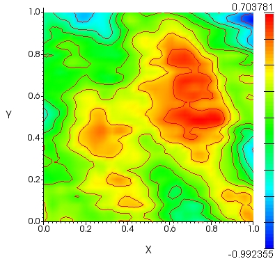
Contour Plot

A contour plot gives you essentially a “topographic map” of a function. The contours join points on the surface that have the same height. By default contour plots are shaded, in such a way that regions with higher z values are lighter. Contour plots display a field with a 2D mesh. To select this view, use 'contour' in <about><view>.

Style flags for contour plots:

• -color <colormap_name>
• -levels <int>: number of contour levels
• -opacity <float: [0,1]>

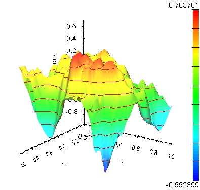
Heightmap Plot

Heightmap plots are used to plot (x,y,z) points in three-dimensional space as a height field surface where the field value (z) is interpreted as the height above the xy-plane. Heightmap plots display a field with a 2D mesh. To select this view, use 'heightmap' in <about><view>.

Style flags for heightmap plots:

• -color <colormap_name>
• -levels <int>: number of contour levels
• -opacity <float: [0,1]>

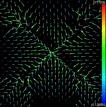
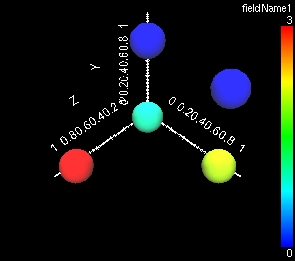
Glyph Plot

The glyph plot places a glyph shape at each point in the mesh. The glyphs may be colored, sized, and/or oriented based on the field values. A common type of glyph plot shows oriented arrows at the points of a vector field, where the arrows point in the direction of the vector at that point in the field. The glyphs may be colored by vector magnitude or a scalar field. Glyph plots display a field with a 2D or 3D mesh. To make use of orienting, coloring and/or sizing by multiple separate fields, use the VTK file data option by including a <component><vtk> element (see above). To select this view, use 'glyphs' in <about><view>.

Style flags for glyphs plot:

• -color <colormap_name>
• -constcolor <color>: color name or hexadecimal color
• -colormode <"scalar"|"vmag"|"vx"|"vy"|"vz"|"constant">
• -cutplaneedges <bool>
• -cutplanelighting <bool>
• -cutplaneopacity <float: [0,1]>
• -cutplanepreinterp <bool>
• -cutplanesvisible <bool>
• -cutplanewireframe <bool>
• -edgecolor <color>: color name or hexadecimal color
• -edges <bool>
• -glyphsvisible <bool>
• -gscale <float>: scaling factor
• -lighting <bool>
• -linewidth <float>
• -normscale <bool>: If set, field data range is normalized to [0,1] before applying scale factor (see -gscale)
• -opacity <float: [0,1]>
• -orientglyphs <bool>: only valid for vector fields. Select a -shape that is not symmetrical in all directions, i.e. don't use a point or sphere shape.
• -outline <bool>
• -ptsize <float>
• -quality <float: [0,10]>: set tesselation quality, defaults to 1.0
• -scalemode <"scalar"|"vmag"|"vcomp"|"off">
• -shape <"arrow"|"cone"|"cube"|"cylinder"|"dodecahedron"|"icosahedron"|"line"|"octahedron"|"point"|"sphere"|"tetrahedron">
• -wireframe <bool>
• -xcutplaneposition <float: [0,100]>
• -xcutplanevisible <bool>
• -ycutplaneposition <float: [0,100]>
• -ycutplanevisible <bool>
• -zcutplaneposition <float: [0,100]>
• -zcutplanevisible <bool>

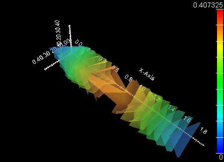
Isosurface Plot

An isosurface plot draws a surface through all the points of the model that have the same value. Isosurfaces plots are surfaces that represent a constant scalar value in a 3D scalar distribution. They are an extension to 2D contour plots. Isosurface plots display a field with a 3D mesh. To select this view, use 'isosurface' in <about><view>.

Style flags for isosurface plot:

• -color <colormap_name>
• -cutplaneedges <bool>
• -cutplanelighting <bool>
• -cutplaneopacity <float: [0,1]>
• -cutplanepreinterp <bool>
• -cutplanesvisible <bool>
• -cutplanewireframe <bool>
• -edgecolor <color>: color name or hexadecimal color
• -edges <bool>
• -isosurfacevisible <bool>
• -levels <int>: number of isosurface levels
• -lighting <bool>
• -linewidth <float>
• -opacity <float>
• -outline <bool>
• -wireframe <bool>
• -xcutplaneposition <float: [0,100]>
• -xcutplanevisible <bool>
• -ycutplaneposition <float: [0,100]>
• -ycutplanevisible <bool>
• -zcutplaneposition <float: [0,100]>
• -zcutplanevisible <bool>

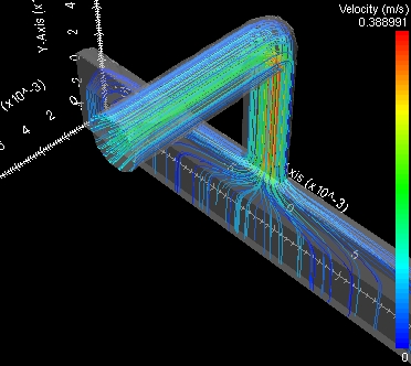
Streamlines Plot

A streamlines plot integrates a vector field to generate streamline paths. Streamlines begin at seed points and represent the forward flow path of particles from the seed points in a steady flow. The streamlines may be colored by the magnitude of the vector field (to show flow speed) or a scalar field. Streamline plots display a field with a 2D or 3D mesh. To make use of coloring by a separate scalar field, use the VTK file data option by including a <component><vtk> element (see above). To select this view, use 'streamlines' in <about><view>.

Additional field elements used to configure this view:

<about><scalars>

Adds metadata about a scalar field that can be used to color the streamlines. This optional element should contain three strings separated by whitespace: a field name, a field label, and units. The field name must match the name of a scalar field in the VTK file data provided in a <component><vtk> element (see above).

<about><vectors>

Adds metadata about the vector field. This optional element should contain three strings separated by whitespace: a field name, a field label, and units. The field name must match the name of a vector field in the VTK file data provided in a <component><vtk> element (see above).

<about><seeds>

This optional element should contain a VTK legacy format file (.vtk). If present, seed points will be randomly distributed in the cells of the provided VTK data set. If not present, the default is to distribute seed points randomly throughout all cells of the field's mesh.

Style flags for streamlines plot:

• -color <colormap_name>
• -constcolor <color>: color name or hexadecimal color
• -edgecolor <color>: color name or hexadecimal color
• -edges <bool>
• -lighting <bool>
• -linewidth <float>
• -mode <"lines"|"ribbons"|"tubes">
• -numseeds <int>
• -opacity <float: [0,1]>
• -seeds <bool>: are seeds visible?
• -seedcolor <color>: color name or hexadecimal color
• -streamlineslength <float>
• -surfacecolor <color>: color name or hexadecimal color
• -surfaceedgecolor <color>: color name or hexadecimal color
• -surfaceedges <bool>
• -surfacelighting <bool>
• -surfaceopacity <float: [0,1]>
• -surfacevisible <bool>
• -surfacewireframe <bool>
• -visible <bool>

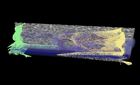
Volume Plot

The volume plot allows the potential to visualize all the data within a three-dimensional volume by mapping scalar values to an opacity and color value. Volume plots display a field with a 3D mesh on a uniform grid. To select this view use either 'nanovis' or 'vtkvolume' in <about><view>. The former is the original nanoHUB volume viewer, the latter is a newer viewer that uses the VTK library.

Style flags for VTK volume plot:

• -color <colormap_name>
• -lighting <bool>
• -opacity <float: [0,1]>
• -outline <bool>
• -visible <bool>

Flow Plot

A flow plot can animate particles through a steady flow field. However, it is anticipated that this view will be deprecated in favor of an enhanced Streamlines view.

How to define a <field> object

For point data fields, there will be one value for each point in the mesh. For cell data fields, there will be one value for each cell in the mesh. The mesh defines the geometry and topology, the values the attributes. For example when displaying a heightmap, the field values will be displayed as the height of the surface at each point in the mesh.

The mesh is a separate <mesh> object. Meshes can be shared among several <field> objects.

<mesh id="m2d">
  <about>
    <label>2D Mesh</label>
  </about>
  <dim>2</dim>
  <units>um</units>
  <hide>yes</hide>
  <grid>
    <xaxis>
      <min>0.0</min>
      <max>1.0</max>
      <numpoints>20</numpoints>
    </xaxis>
    <yaxis>
      <min>-10.0</min>
      <max>10.0</max>
      <numpoints>50</numpoints>
    </yaxis>
  </grid>
</mesh>

<field id="f2d">
  <about>
    <label>2D Field</label>
  </about>
  <units>eV</units>
  <component>
    <mesh>output.mesh(m2d)</mesh>
    <values>0
0
0
0
...
    </values>
  </component>
</field>

In this example, the <mesh> is a 20 x 50 uniform 2D grid with bounds of [0,0um,1.0um] in the X axis and [-10.0um, 10.0um] in the Y axis. The <field> includes a <mesh> attribute pointing to output.mesh(m2d) as the underlying mesh. The values within the field correspond to the points defined in the grid. The first value represents the field at the first mesh point, the second value at the second mesh point, and so forth. In this case, the mesh points are implicitly defined by the grid axes rather than as a list of points. The order of implicit grid points follows the convention of X coordinates changing fastest, then Y coordinates, then Z coordinates. In this case, the mesh is 2D, so we would list point field values according to the grid order: (0,0), (1,0), (2,0)...(19,0), (0,1), (1,1), (2,1)... etc.

You can see working code in the zoo of examples in the field example or on the hub in the directory /apps/rappture/examples/zoo/field.