
| Version 9 (modified by gah, 12 years ago) (diff) |
|---|
<field>
A <field> object represents a set of values defined over a mesh. The mesh is usually a collection of points in space, but it can also represent points in energy, momentum, etc. The mesh is a separate <mesh> object. Meshes can be shared among several <field> objects.
    <field>
        <about>
            <label>3D Field</label>
        </about>
        <component>
            <mesh>output.mymesh</mesh>
            <values>
                0.143588 0.11341 0.104264 0.119749 0.148021 0.195553
                0.209402 0.132308 0.0634601 0.0574183 0.0550705 0.0341862
                0.0239724 0.0343367 0.0490282 0.0629045 0.0890553 0.135098
                0.157703 0.144812 0.15334 0.192826 0.209467 0.199057
                ...
            </values>
        </component>
    </field>
- <about><label>
- This is the label for the output.
- <about><description>
- This is the description of the output. It it reveal when the user hovers over the output in the drop-down list.
- <component><mesh>
- The name of the mesh element. The mesh is a separate <mesh> object.
- <component><values>
- The values of the field. The number of values must match the number of points or cells of the mesh.
There are a variety of ways that fields can be viewed.
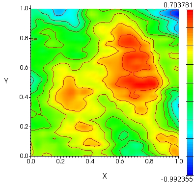
- Contour Plot
- A contour plot gives you essentially a “topographic map” of a function. The contours join points on the surface that have the same height. By default contour plots are shaded, in such a way that regions with higher z values are lighter. Contour plots display a field with a 2D mesh.

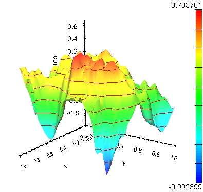
- Surface Plot
- Surface plots are used to plot (x,y,z) points in three-dimensional space as a surface where z is interpreted as the height above the xy-plane. Surfaces plots display a field with a 2D mesh.

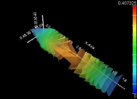
- Isosurface Plot
- An isosurface plot draws a surface through all the points of the model that have the same value. Isosurfaces plots are surfaces that represent a constant scalar value in a 3D scalar distribution. They are an extension to 2D contour plots. Isosurface plots display a field with a 3D mesh.

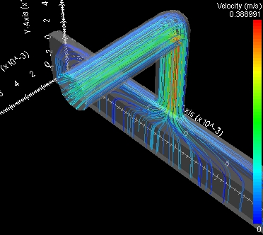
- Streamlines Plot
- A streamline plot is a contour plot of the lines of constant value of the stream function, which represents the trajectories of particles in a steady flow. Isosurface plots display a field with a 3D mesh.

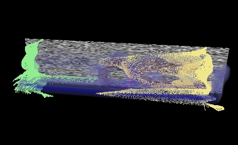
- Volume Plot
- The volume plot allows the potential to visualize all the data within a three-dimensional volume by mapping scalar values to an opacity and color value. Isosurface plots display a field with a 3D mesh on a uniform grid.
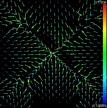
- Flow
There will be one value for each point (or cell) in the mesh. The mesh defines the geometry and topology, the values the attributes. For example when displaying a heightmap, the field values will be displayed as the height of the surface at each point in the mesh.
The mesh is a separate <mesh> object. Meshes can be shared among several <field> objects.
<cloud id="m2d">
  <about>
    <label>2D Mesh</label>
  </about>
  <units>um</units>
  <hide>yes</hide>
  <points>0 0
1 0
2 0
3 0
...
  </points>
</cloud>

<field id="f2d">
  <about>
    <label>2D Field</label>
  </about>
  <component>
    <mesh>output.cloud(m2d)</mesh>
    <values>0
0
0
0
...
    </values>
  </component>
</field>
In this example, the <cloud> contains a series of (x,y) points defining the mesh. The <field> includes a <mesh> attribute pointing to output.cloud(m2d) as the underlying mesh. The values within the field correspond to the points defined in the cloud. The first value represents the field at the first mesh point, the second value at the second mesh point, and so forth.

<mesh id="m3d">
  <about>
    <label>3D Mesh</label>
  </about>
  <units>um</units>
  <hide>yes</hide>
  <node id="0">0 0 0</node>
  <node id="1">1 0 0</node>
  <node id="2">2 0 0</node>
  <node id="3">3 0 0</node>
  ...
  <element id="0">
    <nodes>0 1 5 6 25 26 30 31</nodes>
  </element>
  <element id="1">
    <nodes>1 2 6 7 26 27 31 32</nodes>
  </element>
  ...
</mesh>

<field id="f3d">
  <about>
    <label>3D Field</label>
  </about>
  <component>
    <mesh>output.mesh(m3d)</mesh>
    <values>0
0
0
0
...
    </values>
  </component>
</field>
Meshes can also be defined with explicit connectivity. A <cloud> is just a set of points, which is converted into a mesh automatically via Delaunay triangularization. But a <mesh> element defines a set of points and their connectivity. Each point is defined as a <node> with a specific id. In this example, we have a 3D mesh, so each <node> contains an (x,y,z) coordinate. The mesh also contains a series of <element> objects, which indicate how the nodes are stitched together to form a mesh. The first element is a cube composed of nodes with identifiers (id=) 0, 1, 5, 6, 25, 26, 30, and 31. Note that this mesh has a hole in the center. There is no element defined that connects the inner nodes. This is not an error. It represents a hole in the underlying structure.
The <field> contains a <mesh> attribute that points to output.mesh(m3d) as the underlying mesh. Each value in the field corresponds to a node in the mesh. The first value represents the field at the first node (id=0), the next value at the next node (id=1), and so forth.
NOTE: The newlines after each value in the field and each point in the cloud are significant. They help Rappture differentiate between a scalar and a vector value in a field, or between a 2D point and a 3D point in a cloud.
You can see working code in the zoo of example's in the field example or on the hub in the directory /apps/rappture/examples/zoo/field.
Attachments (8)
- contour.jpg (133.3 KB) - added by gah 12 years ago.
- heightmap.jpg (72.0 KB) - added by gah 12 years ago.
- isosurface.jpg (46.4 KB) - added by gah 12 years ago.
- streamlines.jpg (73.7 KB) - added by gah 12 years ago.
- volume.jpg (47.3 KB) - added by gah 12 years ago.
- flow.jpg (66.4 KB) - added by gah 12 years ago.
-
glyphPlot.jpg
(160.8 KB) -
added by ldelgass 11 years ago.
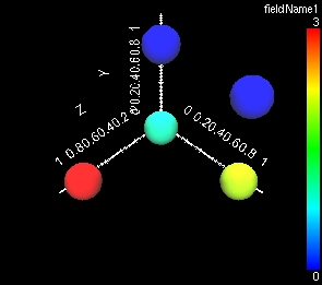
Glyph Plot
- glyphs2.jpg (26.4 KB) - added by ldelgass 10 years ago.
Download all attachments as: .zip